
Effective Resistance and Graph
In this article, I’d like to explain some fun pieces of effective resistance and graph. In a recent paper, I did some research on effective resistance. However, since the research is a bit advanced due to its nature, the size of the audience is far narrowed. Instead of introducing the research, I’d like to shed light on more elementary stuff aiming for wider readers. This will explain how the effective resistance and graph are fun. Also, by looking again the elemental stuff, we might discover some “seeds” that new things can be developed on.
Note: This article is a promotion of our recent paper at ICML.
Graph is a mathematically fun tool. We can interpret a graph from many views, which is one of the reasons why graph is fun. Today, I’d like to play with this fun toy. One view I play with today is an analogy between an electric circuit and a graph. Spoiler alert: we find “distance” over a graph by considering this.
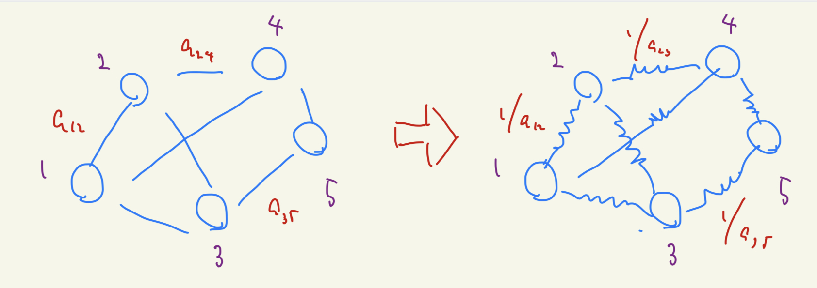
We consider a graph $G=(V,E)$. We construct an electric circuit. We regard the vertices as the endpoints and edges as resistors. When we run electricity over this graph circuit, we want more electricity to run on the edge whose weight is larger. Thus, we design the resistance as an inverse of the weight of the edge.
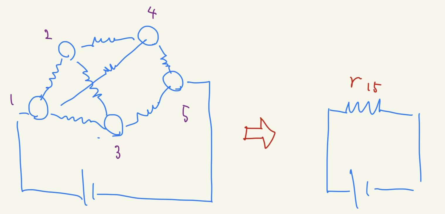
Now, we connect a battery to two endpoints. Then, the whole graph works as a resistance. Although a graph contains multiple resistances over edges, the whole graph can be considered as one resistance, called an effective resistance. This effective resistance may vary by choosing different set of two endpoints.
We want to compute the effective resistance. But how? Recall your high school (or lower education) classroom. How did you compute resistance? If we denote by $S$ an energy over the circuit, by $R$ a resistance, and by $V$ a potential (voltage, the “size” of the battery), we then get $S = V^{2}/R$. We apply the same strategy to this graph case.
The resistance won’t vary even if we connect a different size of battery. Thus, we consider the unit voltage. By seeing $S= 1/R \times V^{2}$, the energy for the potential distribution $\mathbf{x}$ is defined as
\[S_{G,2} (\mathbf{x}) := \sum_{i,j \in V} a_{ij} |x_{i} - x_{j}|^2.\]Note that, again, we consider a circuit whose resistance is defined as an inverse of the edge weight $1/a_{ij}$. We compute the energy of the circuit if we connect the battery $i$ and $j$ that we assume the most stable state when a potential difference between $i$ and $j$ is a unit, such as
\[\min_{\mathbf{x}}\{S_{G,2} (\mathbf{x})\quad \mathrm{s.t}\ x_{i} - x_{j} = 1\}.\]Summarizing the discussion, we define the effective resistance $r_{G,2}(i,j)$ between vertices $i$ and $j$ as
\[r_{G,2}(i,j) := 1/(\min_{\mathbf{x}} \{S_{G,2} (\mathbf{x})\quad \mathrm{s.t}\ x_{i} - x_{j} = 1\}), (*)\]which is again comparable as $S=V^{2}/R$ and hence $R=V^{2}/S$.
I have played enough with this circuit analogy. You are probably an adult, so you might ask, “So what?” This McKinsey style question is always a million-dollar question. You might always be interested in a million dollar. At least, I am.
One significant thing about this effective resistance is that this serves as a distance over a graph. Particularly, the most non-trivial thing is that the effective resistance shows a triangle inequality, such as
\[r_{G,2} (i,j) \leq r_{G,2} (i,\ell) + r_{G,2} (\ell,j).\]This triangle inequality is a classical result, so I won’t go into the details, but Google helps you to prove this. This distance characteristic fascinates many graph researchers. Also, there are many applications of effective resistance, such as clustering, online learning, and computing random spanning trees.
If the effective resistance serves as a distance, we want to compute this as much as possible. Do we need to solve the optimization problem for every pair? Actually, and luckily, no. We have a more convenient way to compute effective resistances. From now on, I borrow the notations of graph $2$-seminorm \(||\mathbf{x}||_{G,2}\) from the equation $(*)$ in my previous post. The details are there, but one important takeaway from the case when $p=2$ is that we can write energy by using the graph 2-seminorm as
\[S_{G,2} (\mathbf{x}) = \|\mathbf{x}\|_{G,2}^{2} = \langle \mathbf{x}, \mathbf{x} \rangle_{L} = \mathbf{x}^{\top}L\mathbf{x} = \sum_{i,j \in V} a_{ij} |x_{i} - x_{j}|^{2},\]where $L$ is an unnormalized graph Laplacian, and $\langle \cdot, \cdot \rangle_{L}$ is an inner product induced by $L$. Using the graph 2-seminorm, the effective resistance is known to be rewritten as
\[r_{G,2} (i,j) = \|L^{+}\mathbf{e}_{i} - L^{+}\mathbf{e}_{j}\|_{G,2}^{2}, \quad (\dagger)\]where $L^{+}$ indicates the pseudoinverse of $L$, and $\mathbf{e}_{i}$ is $i$-th coordinate vector.
The Equation $(\dagger)$ offers a convenient way to compute all the pairs of effective resistance. Instead of solving the optimization problems for all the pairs, we first compute $L^{+}$, and we then compute effective resistance using Equation $(\dagger)$. We can recycle $L^{+}$ for other pairs, saving computation time.
How can we prove the Equation $(\dagger)$? There are many ways to prove this, such as using some elementary circuit way or using Lagrangian multipliers. In this article, I’d like to introduce a way using the Cauchy-Schwarz inequality, that is for the graph 2-seminorm can be written as
\[\langle \mathbf{x}, \mathbf{y} \rangle_{L} \leq \|\mathbf{x}\|_{G,2} \|\mathbf{y}\|_{G,2}.\]Now, we have some fun things. How can we use this Cauchy-Schwarz inequality for the effective resistance defined as Equation $(\ast)$? First, we observe that the constraints of the optimization problem $(\ast)$ as
\[1 = x_{i} - x_{j} = \mathbf{x}^{\top}(\mathbf{e}_{i} - \mathbf{e}_{j} ) = \mathbf{x}^{\top}LL^{+}(\mathbf{e}_{i} - \mathbf{e}_{j} ) = \langle \mathbf{x}, L^{+}\mathbf{e}_{i} - L^{+}\mathbf{e}_{j} \rangle_{L}.\]Thus, plugging this into the Cauchy-Schwarz inequality, I get
\[1 = \langle \mathbf{x}, L^{+}\mathbf{e}_{i} - L^{+}\mathbf{e}_{j} \rangle_{L} \leq \|\mathbf{x}\|_{G,2} \|L^{+}\mathbf{e}_{i} - L^{+}\mathbf{e}_{j}\|_{G,2}.\]Rearranging this, I obtain
\[\|L^{+}\mathbf{e}_{i} - L^{+}\mathbf{e}_{j}\|_{G,2}^{-1} \leq \|\mathbf{x}\|_{G,2}. \quad (\circ)\]So, with the constraint $x_{i} - x_{j} = 1$, \(\|\mathbf{x}\|_{G,2}\) is lower bounded by \(\|L^{+}\mathbf{e}_{i} - L^{+}\mathbf{e}_{j}\|_{G,2}^{-1}\). If the equality of Equation $(\circ)$ holds, we have $(\dagger)$, since
\[(\min_{\mathbf{x}} \{\|\mathbf{x}\|_{G,2}^{2} (\mathbf{x})\quad \mathrm{s.t}\ x_{i} - x_{j} = 1\})^{-1} = \|L^{+}\mathbf{e}_{i} - L^{+}\mathbf{e}_{j}\|_{G,2}^{2}\]Do we have such $\mathbf{x}$ satisfying the equality of $(\circ)$? Yes, when \(\mathbf{x} = (L^{+}\mathbf{e}_{i} - L^{+}\mathbf{e}_{j})/\|L^{+}\mathbf{e}_{i} - L^{+}\mathbf{e}_{j}\|_{G,2}^{2}\), the equality of $(\circ)$ is satisfied. Thus, by considering the Cauchy-Schwarz inequality, we have $(\dagger)$.
Remark that Equation $(\dagger)$ offers a view for a distance over the graph. Each vertex is represented by a vector $L^{+}\mathbf{e}_{i}$, and the effective resistance measures the representation by the norm \(\|\cdot\|_{G,2}^{2}\).
To conclude, this article considers an analogy between graphs and electric circuits. Then, I introduced effective resistance has a significant role due to its distance nature. Moreover, we trace how the Cauchy-Schwarz inequality helps to obtain the exact form of effective resistance $(\dagger)$.
Advert:
Again, like a previous post, if people see the 2-seminorm, it is one of the universe principles that people want to expand to $p$-seminorm. So, can we generalize this discussion to $p$-seminorm, say, $p$-resistance? Does the $p$-resistance show the same triangle inequality? Does there exist some norm \(\|\cdot\|^{\star}\) such that $p$-resistance can be written as \(\|L^{+}\mathbf{e}_{i} - L^{+}\mathbf{e}_{j}\|^{\star}\)?
If you are interested, please read the next post or our paper. Our paper discusses the existence of such a norm of $p$-resistance, by extending Cauchy-Schwarz inequality to Hölder’s inequality.
Citation:
If you find this piece useful, please cite this paper. The proof of Equation $(\dagger)$ using the Cauchy-Schwarz inequality is included as a special case of our Proposition 3.3.
@inproceedings{saito2023multi,
 title={Multi-class Graph Clustering via Approximated Effective $p$-Resistance.},
 author={Saito, Shota and Herbster, Mark},
 booktitle={Proc. ICML},
 pages = {29697--29733},
 year={2023}
}
I have a confession to make. Although I took a course in electric circuits while doing my bachelor’s, I did not understand almost anything.